Plot Examples
Simple test
Ensure your device works with this simple test.
import board
from circuitpython_uplot.plot import Plot

# Setting up the display
display = board.DISPLAY

# Adding the plot area
plot = Plot(0, 0, display.width, display.height)

plot.draw_circle(radius=8, x=120, y=120)

display.show(plot)

Plot Example
Plot some data for x and y
import board
from ulab import numpy as np
from circuitpython_uplot.plot import Plot
from circuitpython_uplot.cartesian import Cartesian

# Setting up the display
display = board.DISPLAY

# Adding the plot area
plot = Plot(0, 0, display.width, display.height)

# Creating some points to graph
x = np.linspace(-4, 4, num=25)
constant = 1.0 / np.sqrt(2 * np.pi)
y = constant * np.exp((-(x**2)) / 2.0)

# Drawing the graph
Cartesian(plot, x, y)

display.show(plot)

Tick Parameters Settings Example
Setting up the ticks parameters
import board
from ulab import numpy as np
from circuitpython_uplot.plot import Plot, color
from circuitpython_uplot.cartesian import Cartesian


# Setting up the display
display = board.DISPLAY

# Setting up the plot area
plot = Plot(
    0,
    0,
    display.width,
    display.height,
    background_color=color.WHITE,
    box_color=color.BLACK,
)

# Setting up tick parameters
plot.tick_params(tickx_height=12, ticky_height=6, tickcolor=color.BLACK, tickgrid=False)
# Seeting some date to plot
x = np.linspace(-4, 4, num=50)
constant = 1.0 / np.sqrt(2 * np.pi)
y = constant * np.exp((-(x**2)) / 2.0)

# Drawing the graph
Cartesian(plot, x, y, line_color=color.BLACK)

# Plotting and showing the plot
display.show(plot)

Integration Example
Example showing different graphics elements integration
import board
from ulab import numpy as np
from uhistogram import Histogram
from circuitpython_uplot.plot import Plot
from circuitpython_uplot.cartesian import Cartesian

# Setting Up the histogram
data = [5, 4, 3, 2, 7, 5, 3, 3, 3, 3, 2, 9, 7, 6]
my_box = Histogram(data, x=50, y=50, width=100, height=100)
my_box.draw()

# Setting up the display
display = board.DISPLAY

# Adding the plot area
plot = Plot(0, 0, display.width, display.height)

# Seeting some date to plot
x = np.linspace(-4, 4, num=50)
constant = 1.0 / np.sqrt(2 * np.pi)
y = constant * np.exp((-(x**2)) / 2.0)

# Plotting and showing the plot
Cartesian(plot, x, y)

# Adding a circle
plot.draw_circle(radius=8, x=120, y=120)

# Showing in the screen
display.show(plot)

Scatter examples
Scatter Example
Scatter plot Example
from random import choice
import board
from ulab import numpy as np
from circuitpython_uplot.plot import Plot
from circuitpython_uplot.scatter import Scatter


# Setting up the display
display = board.DISPLAY

# Adding the plot area
plot = Plot(0, 0, display.width, display.height)

# Setting up tick parameters
plot.tick_params(tickx_height=12, ticky_height=12, tickcolor=0xFF0008, tickgrid=True)
plot.axs_params(axstype="cartesian")
a = np.linspace(1, 100)
b = [choice(a) for _ in a]
Scatter(plot, a, b)

# Plotting and showing the plot
display.show(plot)

Scatter Circle Pointers with diferent Radius
Example showing how to use different radius in the circle pointers
from random import choice
import board
from ulab import numpy as np
from circuitpython_uplot.plot import Plot
from circuitpython_uplot.scatter import Scatter


# Setting up the display
display = board.DISPLAY

# Adding the plot area
plot = Plot(0, 0, display.width, display.height, padding=1)
plot.tick_params(tickx_height=12, ticky_height=12, tickcolor=0x939597, tickgrid=True)

display.show(plot)

a = np.linspace(1, 200, 150)
z = [4, 5, 6, 7, 8]
radi = [choice(z) for _ in a]
b = [choice(a) for _ in a]
Scatter(
    plot, a, b, rangex=[0, 210], rangey=[0, 210], radius=radi, pointer_color=0xF456F3
)

Scatter Pointers Example
Example showing how to use different pointers
from random import choice
import board
from ulab import numpy as np
from circuitpython_uplot.plot import Plot
from circuitpython_uplot.scatter import Scatter


# Setting up the display
display = board.DISPLAY

# Adding the plot area
plot = Plot(0, 0, display.width, display.height)

# Setting up tick parameters
plot.tick_params(tickx_height=12, ticky_height=12, tickcolor=0xFF0008, tickgrid=True)
plot.axs_params(axstype="cartesian")
a = np.linspace(1, 100)
b = [choice(a) for _ in a]
Scatter(plot, a, b)

# Plotting and showing the plot
display.show(plot)

Scatter using different datasets
Example showing how to use different datasets
from random import choice
import board
from ulab import numpy as np
from circuitpython_uplot.plot import Plot
from circuitpython_uplot.scatter import Scatter, Pointer


# Setting up the display
display = board.DISPLAY

# Adding the plot area
plot = Plot(0, 0, display.width, display.height, padding=25)
plot.tick_params(
    tickx_height=12,
    ticky_height=12,
    tickcolor=0x939597,
    tickgrid=True,
    showtext=True,
    decimal_points=0,
)

display.show(plot)

a = np.linspace(4, 200, 50)
z = [4, 5, 6, 7, 8]
radi = [choice(z) for _ in a]
b = [choice(a) for _ in a]
Scatter(
    plot, a, b, rangex=[0, 210], rangey=[0, 210], radius=radi, pointer_color=0xF456F3
)
a = np.linspace(50, 170, 50)
radi = [choice(z) for _ in a]
b = [choice(a) for _ in a]
Scatter(
    plot, a, b, rangex=[0, 210], rangey=[0, 210], radius=radi, pointer_color=0x00FF00
)
a = np.linspace(50, 100, 25)
z = [
    4,
    5,
    6,
]
radi = [choice(z) for _ in a]
b = [int(choice(a) / 1.2) for _ in a]
Scatter(
    plot,
    a,
    b,
    rangex=[0, 210],
    rangey=[0, 210],
    pointer=Pointer.TRIANGLE,
    pointer_color=0x00FFFF,
)

Cartesian examples
Cartesian and Scatter Example
Example showing how to use cartesian and scatter in the same plot
import board
import displayio
from ulab import numpy as np
from table import Table
from circuitpython_uplot.plot import Plot
from circuitpython_uplot.scatter import Scatter
from circuitpython_uplot.cartesian import Cartesian

# In order to run this example you need to install the following libraries:
# - adafruit_display_text
# - adafruit_bitmap_font
# - CircuitPython_TABLE (from https://github.com/jposada202020/CircuitPython_TABLE)

g = displayio.Group()

table_width = 125

# Setting up the display
display = board.DISPLAY

# Adding the plot area
plot = Plot(0, 0, display.width - table_width, display.height, padding=1)
plot.tick_params(tickx_height=12, ticky_height=12, tickcolor=0x939597, tickgrid=True)
plot_table = Plot(
    display.width - table_width - 1, 0, table_width - 1, display.height, padding=1
)

display.show(g)
g.append(plot)
g.append(plot_table)


general_rangex = [0, 17]
general_rangey = [0, 70]

# Creating the values
x = np.array([1, 2, 3, 4, 5, 6, 7, 8, 9, 10, 11, 12, 13, 14, 15])
y = np.array([3, 14, 23, 25, 23, 15, 9, 5, 9, 13, 17, 24, 32, 36, 46])

# Creating the table
# To use the font, create a fonts directory in the root of the CIRCUITPY drive,
# and add the font file from the fonts folder
# fmt: off
my_table = Table(
    10,
    10,
    140,
    315,
    [("-----------", "-----------",)],
    [("Value X", "Value Y",), ("1", "3",), ("2", "14",),("3", "23",),("4", "25",),
     ("5", "23",),("6", "15",),("7", "9",),("8", "5",),("9", "9",),("10", "13",),
     ("11", "17",),("12", "24",),("13", "32",),("14", "36",),
     ("15", "46",)],
    "fonts/LibreBodoniv2002-Bold-10.bdf",
    text_color = 0xFFFFFF,
)
# fmt: on
plot_table.append(my_table)

# Polyfit Curve third degree
z = np.polyfit(x, y, 3)
new_x = np.linspace(0, 16, 50)
fit = z[0] * new_x**3 + z[1] * new_x**2 + z[2] * new_x + z[3]
Cartesian(plot, new_x, fit, rangex=general_rangex, rangey=general_rangey)

# Polyfit Curve Second degree
z = np.polyfit(x, y, 2)
new_x = np.linspace(0, 16, 50)
fit = z[0] * new_x**2 + z[1] * new_x + z[2]
Cartesian(plot, new_x, fit, rangex=general_rangex, rangey=general_rangey)

# Polyfit Curve First degree
z = np.polyfit(x, y, 1)
new_x = np.linspace(0, 16, 50)
fit = z[0] * new_x + z[1]
Cartesian(plot, new_x, fit, rangex=general_rangex, rangey=general_rangey)

# Adding the Scatter Plot
Scatter(
    plot,
    x,
    y,
    rangex=general_rangex,
    rangey=general_rangey,
    pointer="triangle",
    pointer_color=0x00FFFF,
)

# Adding the labels for the Polylines
# change the x and y values to move the text according to your needs
plot.show_text(
    "Polyfit 1",
    x=300,
    y=10,
    anchorpoint=(0.5, 0.0),
    text_color=0x149F14,
    free_text=True,
)
plot.show_text(
    "Polyfit 2",
    x=72,
    y=270,
    anchorpoint=(0.0, 0.0),
    text_color=0x647182,
    free_text=True,
)
plot.show_text(
    "Polyfit 3",
    x=175,
    y=200,
    anchorpoint=(0.5, 0.0),
    text_color=0x7428EF,
    free_text=True,
)

Plot Line Style Example
Plot some data for x and y with different line styles
import board
from ulab import numpy as np
from circuitpython_uplot.plot import Plot
from circuitpython_uplot.cartesian import Cartesian

# Setting up the display
display = board.DISPLAY
plot = Plot(0, 0, display.width, display.height)

# Creating some points to graph
x = np.linspace(-4, 4, num=25)
constant = 1.0 / np.sqrt(2 * np.pi)
y = constant * np.exp((-(x**2)) / 2.0)

# Drawing the graph
Cartesian(
    plot, x, y, rangex=[-5, 5], rangey=[0, 1], line_color=0xFF0000, line_style="- -"
)

# Creating some points to graph
x = np.linspace(-3, 3, num=50)
constant = 2.0 / np.sqrt(2 * np.pi)
y = constant * np.exp((-(x**2)) / 2.0)
Cartesian(
    plot, x, y, rangex=[-5, 5], rangey=[0, 1], line_color=0x00FF00, line_style="."
)


x = np.linspace(-4, 4, num=50)
constant = 2.5 / np.sqrt(2 * np.pi)
y = constant * np.exp((-(x**2)) / 6.5)
Cartesian(
    plot, x, y, rangex=[-5, 5], rangey=[0, 1], line_color=0x123456, line_style="-.-"
)

# Plotting and showing the plot
display.show(plot)

Cartesian fill Example
Cartesian fill example
import board
from ulab import numpy as np
from circuitpython_uplot.plot import Plot
from circuitpython_uplot.cartesian import Cartesian


# Setting up the display
display = board.DISPLAY

# Adding the plot area
plot = Plot(0, 0, display.width - 125, display.height, padding=25)

display.show(plot)

# Creating the values
x = np.array([1, 2, 3, 4, 5, 6, 7, 8, 9, 10, 11, 12, 13, 14, 15])
y = np.array([3, 14, 23, 25, 23, 15, 9, 5, 9, 13, 17, 24, 32, 36, 46])

# Polyfit Curve third degree
z = np.polyfit(x, y, 3)
new_x = np.linspace(0, 15, 50)
fit = z[0] * new_x**3 + z[1] * new_x**2 + z[2] * new_x + z[3]
Cartesian(
    plot,
    new_x,
    fit,
    rangex=[0, 15],
    rangey=[0, 70],
    fill=True,
)

Cartesian Advanced Example
Showing the ability to display to graphs in the same plot with different colors
import board
from ulab import numpy as np
from circuitpython_uplot.plot import Plot
from circuitpython_uplot.cartesian import Cartesian

# Setting up the display
display = board.DISPLAY
plot = Plot(0, 0, display.width, display.height)

# Creating some points to graph
x = np.linspace(-4, 4, num=25)
constant = 1.0 / np.sqrt(2 * np.pi)
y = constant * np.exp((-(x**2)) / 2.0)

# Drawing the graph
Cartesian(plot, x, y, rangex=[-5, 5], rangey=[0, 1], line_color=0xFF0000)

# Creating some points to graph
x = np.linspace(-3, 3, num=50)
constant = 2.0 / np.sqrt(2 * np.pi)
y = constant * np.exp((-(x**2)) / 2.0)
Cartesian(plot, x, y, rangex=[-5, 5], rangey=[0, 1], line_color=0x00FF00)

# Plotting and showing the plot
display.show(plot)

Cartesian Table Example
Example showing how to add a data table to the plot
import displayio
import board
from ulab import numpy as np
from table import Table
from circuitpython_uplot.plot import Plot, color
from circuitpython_uplot.cartesian import Cartesian
from circuitpython_uplot.shade import shade


# Heat Index Example
# To use this example you need to install the Table library from
# https://github.com/jposada202020/CircuitPython_TABLE
# and grab the font from the fonts directory


def heat_index(temp, humidity):
    """
    Inspired by
    https://github.com/CedarGroveStudios/CircuitPython_TemperatureTools

    """

    heat_index_value = (
        -8.78469475556
        + 1.61139411 * temp
        + 2.33854883889 * humidity
        - 0.14611605 * temp * humidity
        - 0.012308094 * temp**2
        - 0.0164248277778 * humidity**2
        + 0.002211732 * temp**2 * humidity
        + 0.00072546 * temp * humidity**2
        - 0.000003582 * temp**2 * humidity**2
    )
    return heat_index_value


# Setting up the display
display = board.DISPLAY

# Adding the plot area
plot = Plot(0, 0, display.width, display.height, padding=5)
# Create a group to hold the objects
g = displayio.Group()

# Creating some points to graph
x = np.linspace(25, 50, num=2)

# Drawing the Shades
shade(
    plot,
    x,
    [25, 25],
    [26.3, 26.3],
    rangex=[25, 50],
    rangey=[25, 60],
    fill_color=0x59FF33,
)
shade(
    plot,
    x,
    [26.3, 26.3],
    [30.5, 30.5],
    rangex=[25, 50],
    rangey=[25, 60],
    fill_color=0xFFFDD0,
)
shade(
    plot,
    x,
    [30.5, 30.5],
    [40.5, 40.5],
    rangex=[25, 50],
    rangey=[25, 60],
    fill_color=0xFFEB99,
)
shade(
    plot,
    x,
    [40.5, 40.5],
    [53.5, 53.5],
    rangex=[25, 50],
    rangey=[25, 60],
    fill_color=0xFFDB58,
)
shade(
    plot,
    x,
    [53.5, 53.5],
    [60, 60],
    rangex=[25, 50],
    rangey=[25, 60],
    fill_color=0xFF9D5C,
)

# Creating some points to graph
x = np.linspace(25, 50, num=25)

# Drawing the graphs
for i in range(40, 110, 10):
    Cartesian(plot, x, heat_index(x, i), rangex=[25, 50], rangey=[25, 60])

g.append(plot)

my_table = Table(
    195,
    215,
    200,
    150,
    [("---------------",)],
    [
        ("Values"),
        ("40%-100%"),
    ],
    "fonts/LibreBodoniv2002-Regular-17.bdf",
    color.BLUE,
)
g.append(my_table)
display.show(g)
Lissajous Curves Example
Example showing how to draw lissajous curves
import math
import board
import displayio
from circuitpython_uplot.plot import Plot, color
from circuitpython_uplot.cartesian import Cartesian

# Inspired by Paul McWhorter Raspberry Pi Pico W LESSON 27: Creating Lissajous Patterns
# on an OLED Display
# And
# https://storm-coder-dojo.github.io/activities/python/curves.html


def create_curve(a=1, b=2, mul_factor=10, delta=3.14 / 2):
    """
    Creates a curve based on the formula
    adapted from https://github.com/JPBotelho/Lissajous-Curve
    Liscense: MIT
    """
    delta = 3.14 / 2
    xvalues = []
    yvalues = []
    for i in range(0, 315):
        t = i * 0.02
        x = mul_factor * math.cos(t * a + delta)
        y = mul_factor * math.sin(t * b)
        xvalues.append(x)
        yvalues.append(y)
        if abs(x - xvalues[0]) + abs(y - yvalues[0]) < 0.01 and i > 1:
            print("iterated " + str(i) + " points")
            break
    return xvalues, yvalues


# Setting up the display
display = board.DISPLAY
plot = Plot(0, 0, display.width // 2, display.height // 2, padding=1)
plot2 = Plot(240, 0, display.width // 2, display.height // 2, padding=1)
plot3 = Plot(0, 160, display.width // 2, display.height // 2, padding=1)
plot4 = Plot(240, 160, display.width // 2, display.height // 2, padding=1)
g = displayio.Group()
g.append(plot)
g.append(plot2)
g.append(plot3)
g.append(plot4)

# Plotting and showing the plot
display.show(g)


# Some Variables
factor = 10
separation = 2

# Creating the Plots
x_number_list, y_number_list = create_curve(1, 2, 10)
Cartesian(
    plot,
    x_number_list,
    y_number_list,
    rangex=[-factor - separation, factor + separation],
    rangey=[-factor - separation, factor + separation],
    line_color=color.GRAY,
)

x_number_list, y_number_list = create_curve(3, 2, 10)
Cartesian(
    plot2,
    x_number_list,
    y_number_list,
    rangex=[-factor - separation, factor + separation],
    rangey=[-factor - separation, factor + separation],
    line_color=color.YELLOW,
)

x_number_list, y_number_list = create_curve(3, 4, 10)
Cartesian(
    plot3,
    x_number_list,
    y_number_list,
    rangex=[-factor - separation, factor + separation],
    rangey=[-factor - separation, factor + separation],
    line_color=color.TEAL,
)

x_number_list, y_number_list = create_curve(5, 4, 10)
Cartesian(
    plot4,
    x_number_list,
    y_number_list,
    rangex=[-factor - separation, factor + separation],
    rangey=[-factor - separation, factor + separation],
    line_color=color.ORANGE,
)

Cartesian Polar Plots Example
Example showing how to draw polar plots using Cartesian
import board
import displayio
import ulab.numpy as np
from circuitpython_uplot.plot import Plot, color
from circuitpython_uplot.cartesian import Cartesian

# Inspired by
# https://github.com/CodeDrome/polar-plots-python

# pylint: disable=dangerous-default-value
# Setting up the display
display = board.DISPLAY
plot = Plot(0, 0, display.width // 2, display.height // 2, padding=1)
plot2 = Plot(240, 0, display.width // 2, display.height // 2, padding=1)
plot3 = Plot(0, 160, display.width // 2, display.height // 2, padding=1)
plot4 = Plot(240, 160, display.width // 2, display.height // 2, padding=1)
g = displayio.Group()
g.append(plot)
g.append(plot2)
g.append(plot3)
g.append(plot4)

# Plotting and showing the plot
display.show(g)


def rose_function(n=3, angle_range=[0, 360], radius=30):
    """
    Rose function
    :param int n: Node number. Defaults to 3
    :param list angle_range: angle range to be plot. Defaults to [0, 360]
    :param int radius: radius of the rose function. Defatuls to 30
    """
    test = np.linspace(angle_range[0], angle_range[1], angle_range[1] - angle_range[0])
    radians = np.radians(test)

    return (
        np.cos(radians) * np.sin(radians * n) * radius,
        np.sin(radians) * np.sin(radians * n) * radius,
    )


def spiral_function(a=1, b=3, angle_range=[0, 720]):
    """
    Spiral Graph
    :param int a: spiral's rotation. Defaults to 1
    :param int b: distance between the lines. Defaults to 3
    :param list angle_range: angle range to be plot. Defaults: [0, 720]
    """

    test = np.linspace(angle_range[0], angle_range[1], angle_range[1] - angle_range[0])
    radians = np.radians(test)

    distance = a + b * radians

    return np.cos(radians) * distance, np.sin(radians) * distance


def cardioid_function(angle_range=[0, 360], radius=35):
    """
    Cardiod Function
    :param list angle_range: angle range to be plot. Defaults: [0, 360]
    :param int radius: Radius of the cardiod plot

    """
    test = np.linspace(angle_range[0], angle_range[1], angle_range[1] - angle_range[0])
    radians = np.radians(test)
    distance = (1 + np.cos(radians)) * radius

    return np.cos(radians) * distance, np.sin(radians) * distance


def circle_function(angle_range=[0, 360], radius=35):
    """
    Circle function
    :param list angle_range: angle range to be plot. Defaults: [0, 360]
    :param int radius: Radius of the cardiod plot
    """
    test = np.linspace(angle_range[0], angle_range[1], angle_range[1] - angle_range[0])
    radians = np.radians(test)
    return np.cos(radians) * radius, np.sin(radians) * radius


x, y = rose_function(n=3, angle_range=[0, 360], radius=35)
Cartesian(plot, x, y, rangex=[-40, 40], rangey=[-40, 40], line_color=0xE30B5D)

x, y = spiral_function(a=1, b=3, angle_range=[0, 900])
Cartesian(plot2, x, y, rangex=[-50, 50], rangey=[-50, 50], line_color=color.YELLOW)

x, y = cardioid_function(angle_range=[0, 360], radius=35)
Cartesian(plot3, x, y, rangex=[-15, 75], rangey=[-50, 50], line_color=color.TEAL)

x, y = circle_function(angle_range=[0, 360], radius=35)
Cartesian(plot4, x, y, rangex=[-40, 40], rangey=[-40, 40], line_color=color.ORANGE)

Cartesian Trigonometric Plots Example
Example showing how to draw Trigonometrics plots using Cartesian
import board
import displayio
import ulab.numpy as np
from adafruit_bitmap_font import bitmap_font
from adafruit_display_text import bitmap_label
from circuitpython_uplot.plot import Plot
from circuitpython_uplot.cartesian import Cartesian

font_file = "fonts/LeagueSpartan-Bold-16.bdf"
font_to_use = bitmap_font.load_font(font_file)

g = displayio.Group()
text = "Sin(x)"
text_area = bitmap_label.Label(font_to_use, text=text, color=0x149F14)
text_area.x = 60
text_area.y = 15
# board.DISPLAY.show(text_area)

text2 = "Cos(x)"
text2_area = bitmap_label.Label(font_to_use, text=text2, color=0x647182)
text2_area.x = 135
text2_area.y = 135

display = board.DISPLAY
# Compute the x and y coordinates for points on a sine curve
x = np.arange(0, 3 * np.pi, 0.1)
y = np.sin(x)
y2 = np.cos(x)

plot = Plot(0, 0, display.width // 2, display.height // 2, padding=1)
Cartesian(plot, x, y, rangex=[0, 10], rangey=[-1.1, 1.1])
Cartesian(plot, x, y2, rangex=[0, 10], rangey=[-1.1, 1.1])

g.append(plot)
g.append(text_area)
g.append(text2_area)

display.show(g)

Cartesian Animation Example
Cartesian animation example
import time
from random import choice
import displayio
import terminalio
import board
from adafruit_display_text import label
from circuitpython_uplot.plot import Plot, color
from circuitpython_uplot.cartesian import Cartesian

# Setting up the display
display = board.DISPLAY

plot = Plot(0, 0, display.width, display.height)
g = displayio.Group()

DISPLAY_WIDTH = 200
DISPLAY_HEIGHT = 200
FOREGROUND_COLOR = color.BLACK
BACKGROUND_COLOR = color.WHITE

background_bitmap = displayio.Bitmap(DISPLAY_WIDTH, DISPLAY_HEIGHT, 1)
# Map colors in a palette
palette = displayio.Palette(1)
palette[0] = BACKGROUND_COLOR
# Create a Tilegrid with the background and put in the displayio group
t = displayio.TileGrid(background_bitmap, pixel_shader=palette)
g.append(t)

text_temperature = label.Label(terminalio.FONT, color=FOREGROUND_COLOR, scale=3)
text_temperature.anchor_point = 0.0, 0.0
text_temperature.anchored_position = 25, 0
g.append(text_temperature)

text_humidity = label.Label(terminalio.FONT, color=FOREGROUND_COLOR, scale=3)
text_humidity.anchor_point = 0.0, 0.0
text_humidity.anchored_position = 130, 0
g.append(text_humidity)


plot_1 = Plot(
    0,
    50,
    200,
    60,
    padding=1,
    show_box=True,
    box_color=color.BLACK,
    background_color=color.WHITE,
)

plot_2 = Plot(
    0,
    180,
    200,
    60,
    padding=1,
    show_box=True,
    box_color=color.BLACK,
    background_color=color.WHITE,
)
plot_1.tick_params(
    tickx_height=4, ticky_height=4, show_ticks=True, tickcolor=color.BLACK
)
plot_2.tick_params(
    tickx_height=4, ticky_height=4, show_ticks=True, tickcolor=color.BLACK
)


temperatures = [26, 25, 24, 23, 28]
humidity = [66, 67, 71, 79]
x = list(range(0, 144, 1))
temp_y = [choice(temperatures) for _ in x]
humidity_y = [choice(humidity) for _ in x]

g.append(plot_1)
g.append(plot_2)

display.show(g)
display.refresh()

for i, element in enumerate(x):
    Cartesian(
        plot_1,
        x[0:i],
        temp_y[0:i],
        rangex=[0, 143],
        rangey=[0, 40],
        fill=False,
        line_color=color.BLACK,
        logging=True,
    )
    Cartesian(
        plot_2,
        x[0:i],
        humidity_y[0:i],
        rangex=[0, 143],
        rangey=[0, 100],
        fill=False,
        line_color=color.BLACK,
        logging=True,
    )
    text_temperature.text = f"{temp_y[i]}"
    text_humidity.text = f"{int(round(humidity_y[i], 0))}%"
    time.sleep(0.1)

Cartesian Koch Snowflake
Cartesian koch snowflake example
# Example adapted to use in CircuitPython and Microplot from
# https://github.com/TheAlgorithms/Python/blob/master/fractals/koch_snowflake.py
# License MIT

import board
from ulab import numpy
from circuitpython_uplot.plot import Plot
from circuitpython_uplot.cartesian import Cartesian


def iterate(initial_vectors: list[numpy.ndarray], steps: int) -> list[numpy.ndarray]:
    vectors = initial_vectors
    for _ in range(steps):
        vectors = iteration_step(vectors)
    return vectors


def iteration_step(vectors: list[numpy.ndarray]) -> list[numpy.ndarray]:
    new_vectors = []
    for i, start_vector in enumerate(vectors[:-1]):
        end_vector = vectors[i + 1]
        new_vectors.append(start_vector)
        difference_vector = end_vector - start_vector
        new_vectors.append(start_vector + difference_vector / 3)
        new_vectors.append(
            start_vector + difference_vector / 3 + rotate(difference_vector / 3, 60)
        )
        new_vectors.append(start_vector + difference_vector * 2 / 3)
    new_vectors.append(vectors[-1])

    return new_vectors


def rotate(vector: numpy.ndarray, angle_in_degrees: float) -> numpy.ndarray:
    theta = numpy.radians(angle_in_degrees)
    c, s = numpy.cos(theta), numpy.sin(theta)
    rotation_matrix = numpy.array(((c, -s), (s, c)))
    return numpy.dot(rotation_matrix, vector)


# Setting up the display
display = board.DISPLAY
plot = Plot(0, 0, 200, 200, padding=0)

# initial triangle of Koch snowflake
VECTOR_1 = numpy.array([0, 0])
VECTOR_2 = numpy.array([0.5, 0.8660254])
VECTOR_3 = numpy.array([1, 0])
INITIAL_VECTORS = [VECTOR_1, VECTOR_2, VECTOR_3, VECTOR_1]
# uncomment for simple Koch curve instead of Koch snowflake
# INITIAL_VECTORS = [VECTOR_1, VECTOR_3]

# Due to memory restrictions the maximum number of iterations is 3.
processed_vectors = iterate(INITIAL_VECTORS, 3)
x_coordinates, y_coordinates = zip(*processed_vectors)

# Adding the Cartesian plot
Cartesian(plot, x_coordinates, y_coordinates)
display.show(plot)

Cartesian Koch Curve
Cartesian koch curve example
# Example adapted to use in CircuitPython and Microplot from
# Heltonbiker
# https://stackoverflow.com/questions/7409938/fractal-koch-curve

import math
import board
from circuitpython_uplot.plot import Plot
from circuitpython_uplot.cartesian import Cartesian

angles = [math.radians(60 * x) for x in range(6)]
sines = [math.sin(x) for x in angles]
cosin = [math.cos(x) for x in angles]


def L(angle, coords, jump):
    return (angle + 1) % 6


def R(angle, coords, jump):
    return (angle + 4) % 6


def F(angle, coords, jump):
    coords.append(
        (coords[-1][0] + jump * cosin[angle], coords[-1][1] + jump * sines[angle])
    )
    return angle


decode = dict(L=L, R=R, F=F)


def koch(steps, length=200, startPos=(0, 0)):
    pathcodes = "F"
    for _ in range(steps):
        pathcodes = pathcodes.replace("F", "FLFRFLF")

    jump = float(length) / (3**steps)
    coords = [startPos]
    angle = 0

    for move in pathcodes:
        angle = decode[move](angle, coords, jump)

    return coords


TOTALWIDTH = 300
display = board.DISPLAY
plot = Plot(0, 0, display.width, display.height, padding=0)
points = koch(5, TOTALWIDTH, (-TOTALWIDTH / 2, 0))
x_coordinates, y_coordinates = zip(*points)

# Adding the Cartesian plot
Cartesian(plot, x_coordinates, y_coordinates)
display.show(plot)

Bar Examples
Bar Example
Bar example
import board
from circuitpython_uplot.plot import Plot
from circuitpython_uplot.bar import Bar


# Setting up the display
display = board.DISPLAY

plot = Plot(0, 0, display.width, display.height)

# Setting up tick parameters
plot.axs_params(axstype="box")
a = ["a", "b", "c", "d"]
b = [3, 5, 1, 7]
Bar(plot, a, b, 0xFF1000, True)

# Plotting and showing the plot
display.show(plot)

Bar Scale Example
Bar plot example showing how to use the scale
import board
import displayio
from circuitpython_uplot.plot import Plot
from circuitpython_uplot.bar import Bar

# Setting up the display
display = board.DISPLAY

# Creating a group to add the two plots
group = displayio.Group()

# Creating the plot objects
plot_scale1 = Plot(0, 0, 100, 100, 1, scale=1)
plot_scale2 = Plot(125, 0, 100, 100, 1, scale=2)

# Creating the data
a = ["a", "b", "c", "d"]
b = [3, 5, 1, 7]

# Creating the bar plot
Bar(plot_scale1, a, b, 0xFF1000, True, bar_space=8, xstart=10)
Bar(plot_scale2, a, b, 0xFF1000, True, bar_space=4, xstart=5)

# Plotting and showing the plot
group.append(plot_scale1)
group.append(plot_scale2)

display.show(group)

Bar Color Palette Example
Bar plot example showing how to pass a user color Palette
import board
from circuitpython_uplot.plot import Plot, color
from circuitpython_uplot.bar import Bar

# Setting up the display
display = board.DISPLAY

# Configuring display dimensions
DISPLAY_WIDTH = 480
DISPLAY_HEIGHT = 320

# Defining the plot
plot = Plot(
    0,
    0,
    DISPLAY_WIDTH,
    DISPLAY_HEIGHT,
    background_color=color.BLACK,
    padding=10,
    box_color=color.BLACK,
)

# Dummy data to plot
activities_latest_heart_value = [55, 20, 25, 30, 35, 10]
a = ["a", "b", "c", "d", "e", "f"]

# Creating the Bar Plot
Bar(
    plot,
    a,
    activities_latest_heart_value,
    0xFF1000,
    True,
    color_palette=[0xFF1000, 0x00FF00, 0x0000FF, 0xFFFF00, 0x00FFFF, 0x123456],
)

# Showing the plot
display.show(plot)

Bar plot updating values Example
Bar Plot example showing how to update values for a filled bars bar plot
import time
import board
from circuitpython_uplot.plot import Plot, color
from circuitpython_uplot.bar import Bar

# Setting up the display
display = board.DISPLAY

# Configuring display dimensions
DISPLAY_WIDTH = 480
DISPLAY_HEIGHT = 320

# Defining the plot
plot = Plot(
    0,
    0,
    DISPLAY_WIDTH,
    DISPLAY_HEIGHT,
    background_color=color.BLACK,
    padding=10,
    box_color=color.BLACK,
)

# Dummy data to plot
some_values = [55, 20, 25, 30, 35, 10]
a = ["a", "b", "c", "d", "e", "f"]

add = 1
# Showing the plot
display.show(plot)

# Creating the bar
my_bar = Bar(
    plot,
    a,
    some_values,
    0xFF1000,
    True,
    color_palette=[
        0xFF1000,
        0x00FF00,
        0x0000FF,
        0xFFFF00,
        0x00FFFF,
        0x123456,
    ],
    max_value=100,
)

for i in range(20):
    values_changed = [j + add for j in some_values]
    my_bar.update_values(values_changed)
    add += 1
    time.sleep(0.1)

for i in range(20):
    values_changed = [j + add for j in some_values]
    my_bar.update_values(values_changed)
    add -= 1
    time.sleep(0.1)
Bar plot updating bar colors Example
Bar Plot example showing how to update colors for a filled bars bar plot
import time
import board
from circuitpython_uplot.plot import Plot, color
from circuitpython_uplot.bar import Bar

# Setting up the display
display = board.DISPLAY

# Configuring display dimensions
DISPLAY_WIDTH = 480
DISPLAY_HEIGHT = 320

# Defining the plot
plot = Plot(
    0,
    0,
    DISPLAY_WIDTH,
    DISPLAY_HEIGHT,
    background_color=color.BLACK,
    padding=10,
    box_color=color.WHITE,
)

display.show(plot)

# Dummy data to plot
some_values = [45, 20, 25, 30, 35, 10]
a = ["a", "b", "c", "d", "e", "f"]

# Showing the plot
display.show(plot)

# Creating the bar
my_bar = Bar(
    plot,
    a,
    some_values,
    0xFF1000,
    True,
    projection=False,
    max_value=50,
)
time.sleep(2)
# Changing all the bars to Yellow
my_bar.update_colors(
    [color.YELLOW, color.YELLOW, color.YELLOW, color.YELLOW, color.YELLOW, color.YELLOW]
)

time.sleep(2)

# Changing the 3 bar to Purple
my_bar.update_bar_color(2, color.PURPLE)
Bar 3D Example
Bar 3D example
import board
from circuitpython_uplot.plot import Plot
from circuitpython_uplot.bar import Bar


# Setting up the display
display = board.DISPLAY

plot = Plot(0, 0, display.width, display.height)

# Setting up tick parameters
plot.axs_params(axstype="box")
a = ["a", "b", "c", "d", "e"]
b = [3, 5, 1, 9, 7]

# Creating a 3D bar
Bar(plot, a, b, color=0xFF1000, fill=True, bar_space=30, xstart=70, projection=True)

# Plotting and showing the plot
display.show(plot)

Pie Examples
Pie Example
Pie example
import board
from circuitpython_uplot.plot import Plot
from circuitpython_uplot.pie import Pie


# Setting up the display
display = board.DISPLAY

plot = Plot(0, 0, display.width, display.height)

# Setting up tick parameters
plot.axs_params(axstype="box")
a = [5, 2, 7, 3]

Pie(plot, a)

# Plotting and showing the plot
display.show(plot)

Stackplot Examples
Stackplot Example
Stackplot simple example
import board
from ulab import numpy as np
from circuitpython_uplot.plot import Plot
from circuitpython_uplot.cartesian import Cartesian

# Setting up the display
display = board.DISPLAY
plot = Plot(0, 0, display.width, display.height)

# Creating some points to graph
x = np.linspace(1, 10, num=10)

y = [6, 7, 9, 6, 9, 7, 6, 6, 8, 9]
Cartesian(plot, x, y, rangex=[0, 11], rangey=[0, 12], line_color=0xFF0000, fill=True)

y = [4, 3, 7, 8, 3, 9, 3, 2, 1, 2]
Cartesian(plot, x, y, rangex=[0, 11], rangey=[0, 12], line_color=0xFF00FF, fill=True)

y = [1, 4, 6, 3, 6, 6, 5, 0, 9, 2]
Cartesian(plot, x, y, rangex=[0, 11], rangey=[0, 12], line_color=0x4444FF, fill=True)


display.show(plot)

Fillbetween Examples
Fillbetween Example
Example of fillbetween plot
import board
from ulab import numpy as np
from circuitpython_uplot.plot import Plot
from circuitpython_uplot.fillbetween import Fillbetween


# Setting up the display
display = board.DISPLAY

plot = Plot(0, 0, display.width, display.height)

x = np.linspace(0, 8, num=25)

y1 = x**2 / 2
y2 = 2 + x**2 + 3 * x

Fillbetween(plot, x, y1, y2)

display.show(plot)

Map Examples
Map Example
map simple example
from random import choice
import board
from ulab import numpy as np
from circuitpython_uplot.plot import Plot
from circuitpython_uplot.map import Map


# Setting up the display
display = board.DISPLAY

# Adding the plot area
plot = Plot(0, 0, display.width, display.height, show_box=False)

# Setting some date to plot
x = np.linspace(-4, 4, num=100)
y = 2.0 / np.sqrt(2 * np.pi) * np.exp((-(x**2)) / 4.0)
b = [choice(y) for _ in y]
y1 = np.array(b).reshape((10, 10))

# Plotting and showing the plot
Map(plot, y1, 0xFF0044, 0x4400FF)
# Plotting and showing the plot
display.show(plot)

Logging Examples
Logging Example
Logging example
import displayio
import terminalio
import board
from adafruit_display_text import label
from circuitpython_uplot.plot import Plot, color
from circuitpython_uplot.logging import Logging

# Setting up the display
display = board.DISPLAY

plot = Plot(0, 0, display.width, display.height)
g = displayio.Group()

DISPLAY_WIDTH = 200
DISPLAY_HEIGHT = 200
FOREGROUND_COLOR = color.BLACK
BACKGROUND_COLOR = color.WHITE

background_bitmap = displayio.Bitmap(DISPLAY_WIDTH, DISPLAY_HEIGHT, 1)
# Map colors in a palette
palette = displayio.Palette(1)
palette[0] = BACKGROUND_COLOR
# Create a Tilegrid with the background and put in the displayio group
t = displayio.TileGrid(background_bitmap, pixel_shader=palette)
g.append(t)

text_temperature = label.Label(terminalio.FONT, color=FOREGROUND_COLOR, scale=3)
text_temperature.anchor_point = 0.0, 0.0
text_temperature.anchored_position = 25, 0
g.append(text_temperature)

text_humidity = label.Label(terminalio.FONT, color=FOREGROUND_COLOR, scale=3)
text_humidity.anchor_point = 0.0, 0.0
text_humidity.anchored_position = 130, 0
g.append(text_humidity)

plot_1 = Plot(
    0,
    50,
    200,
    60,
    padding=1,
    show_box=True,
    box_color=color.BLACK,
    background_color=color.WHITE,
)

plot_1.tick_params(
    tickx_height=4, ticky_height=4, show_ticks=True, tickcolor=color.BLACK
)

x = [10, 20, 30, 40, 50]
temp_y = [26, 25, 24, 23, 28]

g.append(plot_1)

display.show(g)
display.refresh()

dist = 3

Logging(
    plot_1,
    x[0:dist],
    temp_y[0:dist],
    rangex=[0, 200],
    rangey=[0, 100],
    line_color=color.BLACK,
    ticksx=[10, 50, 80, 100],
    ticksy=[15, 30, 45, 60],
)

text_temperature.text = "{}C".format(temp_y[dist])
Logging Fill Example
Logging fill example
import displayio
import board
from circuitpython_uplot.plot import Plot, color
from circuitpython_uplot.logging import Logging

# Setting up the display
display = board.DISPLAY

group = displayio.Group()


palette = displayio.Palette(1)
palette[0] = 0x000000

plot_1 = Plot(
    0,
    0,
    150,
    60,
    padding=1,
    show_box=True,
    box_color=color.BLACK,
    background_color=color.TEAL,
    scale=2,
)

plot_1.tick_params(
    tickx_height=4, ticky_height=4, show_ticks=True, tickcolor=color.BLACK
)

plot_2 = Plot(
    0,
    150,
    300,
    120,
    padding=1,
    show_box=True,
    box_color=color.BLACK,
    background_color=color.YELLOW,
    scale=1,
)

plot_2.tick_params(
    tickx_height=4, ticky_height=4, show_ticks=True, tickcolor=color.BLACK
)

x = [10, 20, 30, 40, 50]
temp_y = [26, 25, 24, 23, 28]

Logging(
    plot_1,
    x,
    temp_y,
    rangex=[0, 200],
    rangey=[0, 50],
    line_color=color.BLACK,
    ticksx=[10, 50, 80, 100],
    ticksy=[15, 30, 45, 60],
    fill=True,
)
Logging(
    plot_2,
    x,
    temp_y,
    rangex=[0, 200],
    rangey=[0, 50],
    line_color=color.BLACK,
    ticksx=[10, 50, 80, 100],
    ticksy=[15, 30, 45, 60],
    fill=True,
)

group.append(plot_1)
group.append(plot_2)

display.show(group)

Logging Changing Values Example
This example shows how to redraw new_values in the same plot
import time
import displayio
import board
from circuitpython_uplot.plot import Plot, color
from circuitpython_uplot.logging import Logging

# Setting up the display
display = board.DISPLAY

plot = Plot(0, 0, display.width, display.height)
g = displayio.Group()

DISPLAY_WIDTH = 200
DISPLAY_HEIGHT = 200
FOREGROUND_COLOR = color.BLACK
BACKGROUND_COLOR = color.WHITE

background_bitmap = displayio.Bitmap(DISPLAY_WIDTH, DISPLAY_HEIGHT, 1)
# Map colors in a palette
palette = displayio.Palette(1)
palette[0] = BACKGROUND_COLOR
# Create a Tilegrid with the background and put in the displayio group
t = displayio.TileGrid(background_bitmap, pixel_shader=palette)
g.append(t)


plot_1 = Plot(
    0,
    50,
    200,
    60,
    padding=1,
    show_box=True,
    box_color=color.BLACK,
    background_color=color.WHITE,
)

plot_1.tick_params(
    tickx_height=4, ticky_height=4, show_ticks=True, tickcolor=color.BLACK
)

x = [10, 20, 30, 40, 50, 60, 70, 80, 90, 100]
temp_y = [26, 25, 24, 23, 28, 24, 54, 76, 34, 23]

g.append(plot_1)

display.show(g)
display.refresh()

my_log = Logging(
    plot_1,
    x,
    temp_y,
    rangex=[0, 200],
    rangey=[0, 100],
    line_color=color.BLACK,
    ticksx=[10, 50, 80, 100],
    ticksy=[15, 30, 45, 60],
)


for i in range(2):
    for i in range(len(x)):
        my_log.draw_points(plot_1, x[0:i], temp_y[0:i])
        time.sleep(1)
Logging with Table Example
This example shows how to add a data table to the plot
import time
import displayio
import board
from table import Table
from circuitpython_uplot.plot import Plot, color
from circuitpython_uplot.logging import Logging

# Create a display object
display = board.DISPLAY

# Create a table object
# To use the font, create a fonts directory in the root of the CIRCUITPY drive,
# and add the font file from the fonts folder
my_table = Table(
    95,
    65,
    200,
    150,
    [("-------------", "-----------")],
    [
        ("Range", "Values"),
        ("Temp", "-50-125"),
        ("Humidity", "0-100%"),
    ],
    "fonts/LibreBodoniv2002-Bold-10.bdf",
    color.BLUE,
)

# Create a group to hold the objects
g = displayio.Group()

# Create a plot object
plot_1 = Plot(
    0,
    50,
    200,
    160,
    padding=1,
    show_box=True,
    box_color=color.BLACK,
    background_color=color.WHITE,
)

plot_1.tick_params(
    tickx_height=4, ticky_height=4, show_ticks=True, tickcolor=color.BLUE
)

# Defining some data
x = [10, 20, 30, 40, 50, 60, 70, 80, 90, 100]
temp_y = [26, 25, 24, 23, 28, 24, 54, 76, 34, 23]

# Create a logging object
my_log = Logging(
    plot_1,
    x,
    temp_y,
    rangex=[0, 200],
    rangey=[0, 100],
    line_color=color.BLACK,
    ticksx=[10, 50, 80, 100],
    ticksy=[15, 30, 45, 60],
)

# Append the objects to the group
g.append(plot_1)
g.append(my_table)
# Show the group
display.show(g)

for _ in range(2):
    for i in range(len(x)):
        my_log.draw_points(plot_1, x[0:i], temp_y[0:i])
        time.sleep(1)

Logging Animation Example
This example shows how to animate a plot
import time
import random
import board
from circuitpython_uplot.plot import Plot, color
from circuitpython_uplot.logging import Logging

# Setting up the display
display = board.DISPLAY
display.auto_refresh = False

# Drawing the graph
my_plot = Plot(
    140,
    60,
    200,
    200,
    padding=25,
    show_box=True,
    box_color=color.WHITE,
)

# Setting the tick parameters
my_plot.tick_params(
    tickx_height=4,
    ticky_height=4,
    show_ticks=True,
    tickcolor=color.TEAL,
    showtext=True,
)

# Creating the x and y data
x = [
    10,
    20,
    30,
    40,
    50,
    60,
    70,
    80,
    90,
    100,
    110,
    120,
    130,
    140,
    150,
    160,
    170,
    180,
    190,
]
y = [26, 22, 24, 30, 28, 35, 26, 25, 24, 23, 20, 27, 26, 33, 24, 23, 19, 27, 26]

# Creating the random numbers
random_numbers = [19, 22, 35, 33, 24, 26, 28, 37]


display.show(my_plot)
display.refresh()

dist = 1

# Creating the loggraph
my_loggraph = Logging(
    my_plot,
    x[0:dist],
    y[0:dist],
    rangex=[0, 210],
    rangey=[0, 110],
    line_color=color.BLUE,
    ticksx=[25, 50, 75, 100, 125, 150, 175, 200],
    ticksy=[25, 50, 75, 100],
)

# Showing the loggraph
for _ in range(20):
    if dist > len(x):
        y.pop(0)
        y.append(random.choice(random_numbers))

    my_loggraph.draw_points(my_plot, x[0:dist], y[0:dist])
    display.refresh()
    dist += 1
    time.sleep(0.5)
Logging Animation Example
This example shows how to add limits to our plot
import time
import random
import board
from circuitpython_uplot.plot import Plot, color
from circuitpython_uplot.logging import Logging

# Setting up the display
display = board.DISPLAY
display.auto_refresh = False

# Drawing the graph
my_plot = Plot(
    140,
    60,
    200,
    200,
    show_box=True,
    box_color=color.WHITE,
)

# Setting the tick parameters
my_plot.tick_params(
    tickx_height=4,
    ticky_height=4,
    show_ticks=True,
    tickcolor=color.TEAL,
    showtext=True,
)

# Creating the x and y data
x = [
    10,
    20,
    30,
    40,
    50,
    60,
    70,
    80,
    90,
    100,
    110,
    120,
    130,
    140,
    150,
    160,
    170,
    180,
    190,
]
y = [26, 32, 34, 30, 28, 35, 46, 65, 37, 23, 40, 27, 26, 36, 44, 53, 69, 27, 26]

# Creating the random numbers
random_numbers = [32, 34, 45, 65, 24, 40, 18, 27]


display.show(my_plot)
display.refresh()

dist = 1

# Creating the loggraph
my_loggraph = Logging(
    my_plot,
    x[0:dist],
    y[0:dist],
    rangex=[0, 210],
    rangey=[0, 110],
    line_color=color.BLUE,
    ticksx=[25, 50, 75, 100, 125, 150, 175, 200],
    ticksy=[25, 50, 75, 100],
    limits=[30, 60],
)

# Showing the loggraph
for i in range(45):
    if dist > len(x):
        y.pop(0)
        y.append(random.choice(random_numbers))

    my_loggraph.draw_points(my_plot, x[0:dist], y[0:dist])
    display.refresh()
    dist += 1
    time.sleep(0.5)

Logging with Dial Gauge Library
This example shows how to add limits to our plot
import time
import random
import board
import displayio
from dial_gauge import DIAL_GAUGE
from circuitpython_uplot.plot import Plot, color
from circuitpython_uplot.logging import Logging


# In order to run this example you need to install the following library:
# - CircuitPython_DIAL_GAUGE (from https://github.com/jposada202020/CircuitPython_DIAL_GAUGE)

rangey_values = [0, 110]

display = board.DISPLAY
display.auto_refresh = False
my_plot = Plot(0, 0, display.width // 2, display.height // 2)
plot2 = Plot(display.width // 2, 0, display.width // 2, display.height // 2)

my_dial = DIAL_GAUGE(60, 50, 60, 40, range_values=rangey_values, color=color.BLUE)

plot2.append(my_dial)

g = displayio.Group()
g.append(my_plot)
g.append(plot2)
display.show(g)


my_plot.tick_params(
    tickx_height=4,
    ticky_height=4,
    show_ticks=True,
    tickcolor=color.TEAL,
    showtext=True,
)

# Creating the x and y data
x = [
    10,
    20,
    30,
    40,
    50,
    60,
    70,
    80,
    90,
    100,
    110,
    120,
    130,
    140,
    150,
    160,
    170,
    180,
    190,
]
y = []

# Creating the random numbers
random_numbers = [32, 34, 45, 65, 24, 40, 18, 27]


# display.show(my_plot)
display.refresh()

dist = 0

# Creating the loggraph
my_loggraph = Logging(
    my_plot,
    x[0:dist],
    y[0:dist],
    rangex=[0, 210],
    rangey=rangey_values,
    line_color=color.BLUE,
    ticksx=[25, 50, 75, 100, 125, 150, 175, 200],
    ticksy=[25, 50, 75, 100],
    limits=[30, 60],
)

# Showing the loggraph
for i in range(150):
    if dist > len(x):
        y.pop(0)

    update_value = random.choice(random_numbers)
    y.append(update_value)

    my_loggraph.draw_points(my_plot, x[0:dist], y[0:dist])

    if dist > len(x):
        my_dial.update(update_value)
    else:
        my_dial.update(y[i])
    display.refresh()
    dist += 1
    time.sleep(0.5)

SVG Examples
SVG Images examples
SVG Images example
import board
from circuitpython_uplot.plot import Plot, color
from circuitpython_uplot.svg import SVG
from circuitpython_uplot.icons import FULL, Humidity, Temperature, Temperature2


# Setting up the display
display = board.DISPLAY

plot = Plot(0, 0, display.width, display.height)
SVG(plot, FULL, 50, 50, 2, color.YELLOW)
SVG(plot, Humidity, 150, 50, 2, color.TEAL)
SVG(plot, Temperature, 250, 50, 2, color.GREEN)

SVG(plot, Temperature2, 300, 50, 0.25, color.BLUE)
display.show(plot)

Shade Examples
Shade examples
Shade example
import board
from ulab import numpy as np
from circuitpython_uplot.plot import Plot
from circuitpython_uplot.cartesian import Cartesian
from circuitpython_uplot.shade import shade

# This example is based in the following Library
# https://github.com/CedarGroveStudios/CircuitPython_TemperatureTools
# And this Wikipedia Article
# https://en.wikipedia.org/wiki/Heat_index


# Setting up the display
display = board.DISPLAY

# Adding the plot area
plot = Plot(0, 0, display.width, display.height, padding=5)


def heat_index(temp, humidity):
    """
    Inspired by
    https://github.com/CedarGroveStudios/CircuitPython_TemperatureTools

    """

    heat_index_value = (
        -8.78469475556
        + 1.61139411 * temp
        + 2.33854883889 * humidity
        - 0.14611605 * temp * humidity
        - 0.012308094 * temp**2
        - 0.0164248277778 * humidity**2
        + 0.002211732 * temp**2 * humidity
        + 0.00072546 * temp * humidity**2
        - 0.000003582 * temp**2 * humidity**2
    )
    return heat_index_value


x = np.linspace(25, 50, num=2)

# Drawing the Shades
shade(
    plot,
    x,
    [25, 25],
    [26.3, 26.3],
    rangex=[25, 50],
    rangey=[25, 60],
    fill_color=0x59FF33,
)
shade(
    plot,
    x,
    [26.3, 26.3],
    [30.5, 30.5],
    rangex=[25, 50],
    rangey=[25, 60],
    fill_color=0xFFFDD0,
)
shade(
    plot,
    x,
    [30.5, 30.5],
    [40.5, 40.5],
    rangex=[25, 50],
    rangey=[25, 60],
    fill_color=0xFFEB99,
)
shade(
    plot,
    x,
    [40.5, 40.5],
    [53.5, 53.5],
    rangex=[25, 50],
    rangey=[25, 60],
    fill_color=0xFFDB58,
)
shade(
    plot,
    x,
    [53.5, 53.5],
    [60, 60],
    rangex=[25, 50],
    rangey=[25, 60],
    fill_color=0xFF9D5C,
)

# Creating some points to graph
x = np.linspace(25, 50, num=25)

# Drawing the graphs
for i in range(40, 110, 10):
    Cartesian(plot, x, heat_index(x, i), rangex=[25, 50], rangey=[25, 60])

display.show(plot)

Polar Plot Examples
Polar example
Show how to use the Polar Plot
import board
import ulab.numpy as np
from circuitpython_uplot.plot import Plot, color
from circuitpython_uplot.polar import Polar

# Setting up the display
display = board.DISPLAY
plot = Plot(10, 10, 250, 250, padding=0, show_box=False)

# Creating the data
r = np.arange(0, 2, 0.01)
theta = 2 * np.pi * r

# Plotting and showing the plot
Polar(plot, theta, r, rangex=[-2, 2], rangey=[-2, 2], line_color=color.ORANGE)
display.show(plot)

Polar Advanced Example
Polar Advanced example
import board
import ulab.numpy as np
import displayio
from circuitpython_uplot.plot import Plot, color
from circuitpython_uplot.polar import Polar


# Setting up the display
display = board.DISPLAY
g = displayio.Group()

# Drawing an Ellipse
theta = np.arange(0, 2 * np.pi, 0.01)
a = 2
b = 1
r = (a * b) / np.sqrt((a * np.sin(theta)) ** 2 + (b * np.cos(theta)) ** 2)

plot = Plot(0, 0, 160, 160, padding=0, show_box=False)
Polar(plot, theta, r, rangex=[-2, 2], rangey=[-2, 2], line_color=color.ORANGE)
g.append(plot)

# Drawing an Spiral
r2 = 2 * np.pi * theta + 4.5
plot2 = Plot(0, 160, 160, 160, padding=0, show_box=False)
Polar(plot2, r2, theta, rangex=[-2, 2], rangey=[-2, 2], line_color=color.ORANGE)
g.append(plot2)

# Drawing a Star
rhos = 2 + np.cos(5 * theta)
plot3 = Plot(160, 0, 160, 160, padding=0, show_box=False)
Polar(
    plot3,
    theta,
    rhos,
    rangex=[-4, 4],
    rangey=[-4, 4],
    line_color=color.ORANGE,
    radius_ticks=[2.0, 4.0],
)
g.append(plot3)

# Drawing a more dense Spiral
rhos = (np.pi / 2) * np.cos(3 * theta)
plot5 = Plot(320, 0, 160, 160, padding=0, show_box=False)
Polar(
    plot5,
    rhos,
    theta,
    rangex=[-4, 4],
    rangey=[-4, 4],
    line_color=color.ORANGE,
    radius_ticks=[2.0, 4.0],
)
g.append(plot5)

# Drawing a funky Shape
rhos = (np.pi / 2) * theta**2
plot4 = Plot(160, 160, 160, 160, padding=0, show_box=False)
Polar(
    plot4,
    rhos,
    theta,
    rangex=[-4, 4],
    rangey=[-4, 4],
    line_color=color.ORANGE,
    radius_ticks=[2.0, 4.0],
)
g.append(plot4)

# Show the Display
display.show(g)

Others
Sparkline Animation Example
Sparkline animation example
import time
import board
from ulab import numpy as np
from adafruit_display_shapes.sparkline import Sparkline
from circuitpython_uplot.plot import Plot, color


# Setting up the display
display = board.DISPLAY

# Adding the plot area
plot = Plot(0, 0, display.width, display.height)

# 500 linearly spaced numbers
x = np.linspace(-10 * np.pi, 10 * np.pi, 500)

# the function, which is y = sin(x) here
y = np.sin(x)

# Creating the sparkline
sparkline = Sparkline(
    width=200,
    height=200,
    max_items=80,
    y_min=np.min(y),
    y_max=np.max(y),
    x=100,
    y=40,
    color=color.TEAL,
)

# Adding shapes to the plot
plot.append(sparkline)

# Plotting and showing the plot
display.show(plot)

for element in y:
    display.auto_refresh = False
    sparkline.add_value(element)
    display.auto_refresh = True

    time.sleep(0.1)
Display_shapes Example
Display Shapes integration example
import board
from adafruit_display_shapes.polygon import Polygon
from adafruit_display_shapes.roundrect import RoundRect
from circuitpython_uplot.plot import Plot

# Setting up the display
display = board.DISPLAY

# Adding the plot area
plot = Plot(0, 0, display.width, display.height)

# Setting up tick parameters
plot.tick_params(tickx_height=12, ticky_height=12, tickcolor=0xFF0008, tickgrid=True)
plot.axs_params(axstype="box")

# Creating some shapes to show
polygon = Polygon(
    [
        (255, 40),
        (262, 62),
        (285, 62),
        (265, 76),
        (275, 100),
        (255, 84),
        (235, 100),
        (245, 76),
        (225, 62),
        (248, 62),
    ],
    outline=0x0000FF,
)

roundrect = RoundRect(30, 30, 61, 81, 10, fill=0x0, outline=0xFF00FF, stroke=6)

# Adding shapes to the plot
plot.append(polygon)
plot.append(roundrect)

# Plotting and showing the plot
display.show(plot)

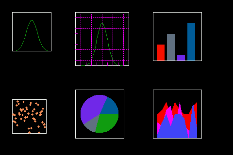
Advanced Example
plot different ulements in a single display
from random import choice
import board
import displayio
from ulab import numpy as np
from circuitpython_uplot.plot import Plot
from circuitpython_uplot.bar import Bar
from circuitpython_uplot.scatter import Scatter
from circuitpython_uplot.pie import Pie
from circuitpython_uplot.cartesian import Cartesian


display = board.DISPLAY
plot = Plot(0, 0, display.width, display.height, show_box=False)

group = displayio.Group()

palette = displayio.Palette(1)
palette[0] = 0xFFFFFF


plot2 = Plot(0, 0, 130, 130)
x = np.linspace(-4, 4, num=25)
constant = 2.0 / np.sqrt(2 * np.pi)
y = constant * np.exp((-(x**2)) / 4.0)
Cartesian(plot2, x, y, rangex=[-5, 5], rangey=[0, 1])
plot.append(plot2)

plot3 = Plot(130, 0, 160, 160)

# Setting up tick parameters
plot3.tick_params(tickx_height=12, ticky_height=12, tickcolor=0xFF00FF, tickgrid=True)

# Seeting some data to plot
x = np.linspace(-4, 4, num=50)
constant = 1.0 / np.sqrt(2 * np.pi)
y = constant * np.exp((-(x**2)) / 2.0)

# Plotting and showing the plot
Cartesian(plot3, x, y, rangex=[-5, 5], rangey=[0, 0.5])
plot.append(plot3)

plot4 = Plot(290, 0, 150, 150)

# Setting up tick parameters
plot4.axs_params(axstype="box")
a = ["a", "b", "c", "d"]
b = [3, 5, 1, 7]
Bar(plot4, a, b, 0xFF1000, fill=True)

plot.append(plot4)

plot5 = Plot(0, 180, 120, 120)

# Setting up tick parameters
plot5.axs_params(axstype="cartesian")
a = np.linspace(3, 98)
b = [choice(a) for _ in a]
Scatter(plot5, a, b, rangex=[0, 102], rangey=[0, 102], radius=2)

plot.append(plot5)

plot6 = Plot(130, 160, 150, 150)

# Setting up tick parameters
plot6.axs_params(axstype="box")
a = [5, 2, 7, 3]

Pie(plot6, a, 0, 0)

plot.append(plot6)


plot7 = Plot(290, 160, 150, 150)

# Creating some points to graph
x = np.linspace(1, 10, num=10)

y = [6, 7, 9, 6, 9, 7, 6, 6, 8, 9]
Cartesian(plot7, x, y, rangex=[0, 11], rangey=[0, 12], line_color=0xFF0000, fill=True)

y = [4, 3, 7, 8, 3, 9, 3, 2, 1, 2]
Cartesian(plot7, x, y, rangex=[0, 11], rangey=[0, 12], line_color=0xFF00FF, fill=True)

y = [1, 4, 6, 3, 6, 6, 5, 0, 9, 2]
Cartesian(plot7, x, y, rangex=[0, 11], rangey=[0, 12], line_color=0x4444FF, fill=True)

plot.append(plot7)

# Plotting and showing the plot
display.show(plot)
Uboxplot Example
example of uboxplot integration in a plot
import board
from boxplot import Boxplot
from circuitpython_uplot.plot import Plot


display = board.DISPLAY

plot = Plot(0, 0, display.width, display.height)

plot.tick_params(tickx_height=10, ticky_height=10, tickcolor=0x440008, tickgrid=True)

a = [1, 1, 4, 5, 6, 7, 7, 7, 8, 9, 10, 15, 16, 17, 24, 56, 76, 87, 87]
my_box = Boxplot(a, x=50, y=50, height=100, line_color=0xFF00FF)
my_box.draw()

b = [1, 1, 4, 5, 6, 7, 7, 7, 8, 9, 10, 15, 16, 17, 24]
my_box2 = Boxplot(b, x=90, y=90, height=100, line_color=0x0000FF)
my_box2.draw()

c = [
    1,
    1,
    4,
    5,
    6,
    7,
    7,
    7,
    8,
    9,
    9,
    9,
    9,
    9,
    9,
    9,
    9,
    9,
    9,
    10,
    15,
    15,
    15,
    15,
    16,
    16,
    17,
    23,
    28,
    39,
    41,
    41,
    41,
    43,
]
my_box3 = Boxplot(c, x=150, y=50, height=100, line_color=0x1CFF11)
my_box3.draw()

plot.append(my_box)
plot.append(my_box2)
plot.append(my_box3)
display.show(plot)
